Gallery
Issue Trees
An issue tree is used to divide a large open question into a series of smaller questions that can be answered by rigorous analysis. This movie shows how to create an issue tree, using a simple example.
Credit: Matthew Juniper
Credit: Matthew Juniper
Issue Trees applied to engineering
This movie shows how an issue tree can be applied to an engineering question.
Credit: Matthew Juniper
Credit: Matthew Juniper
Hypothesis trees
A hypothesis tree is used to divide a statement into its components, all of which must be true in order for the research question to be true.
Credit: Matthew Juniper
Credit: Matthew Juniper
Hypothesis Trees applied to engineering
This movie shows how a hypothesis tree can be applied to an engineering question.
Credit: Matthew Juniper
Credit: Matthew Juniper
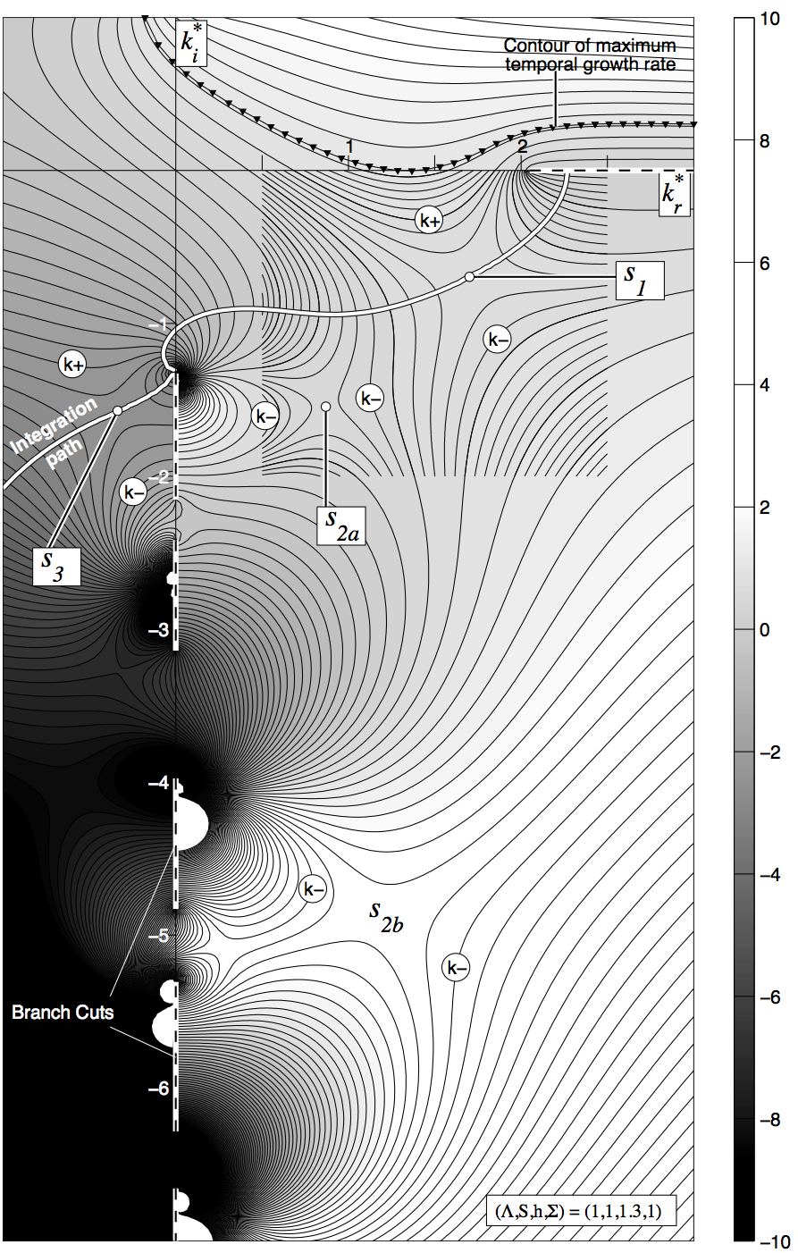
Spatio-temporal stability analysis
This figure shows contours of growth rate (omega_i) in the complex wavenumber (k_r,k_i) plane for a confined planar jet of one fluid within another fluid of the same density. The response to an impulse is found by integrating omega_i along the integration path (white line). In the long time limit, this is dominated by the contributions at the saddle points (white circles). Physically, this is because these points correspond to waves with zero group velocity (because d(omega)/d(k) = 0). These waves remain at the point of impulse and, if they grow in time, dominate the response there. A temporal stability anlaysis can be deduced from this figure by considering a slice of omega(k) through the k_r axis.
Credit: Matthew Juniper
Jump to publication (will be at top of next screen)
Credit: Matthew Juniper
Jump to publication (will be at top of next screen)
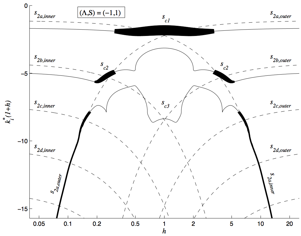
Sinuous instability of confined flows
Cross-stream wavenumber (k_i) of the most unstable wave with zero group velocity as a function of confinement ratio, h, for sinuous motion of a confined wake flow. The thickness of the line is proportional to the growth rate. The dashed lines show the value of k_i for modes in the inner flow and outer flow if the other flow were not present. This shows that the confined flow is most unstable at values of h at which the modes in the inner flow and outer flow have the same cross-stream wavenumber, which is at h=1 for sinuous wake flows.
Credit: Matthew Juniper
Jump to publication (will be at top of next screen)
Credit: Matthew Juniper
Jump to publication (will be at top of next screen)
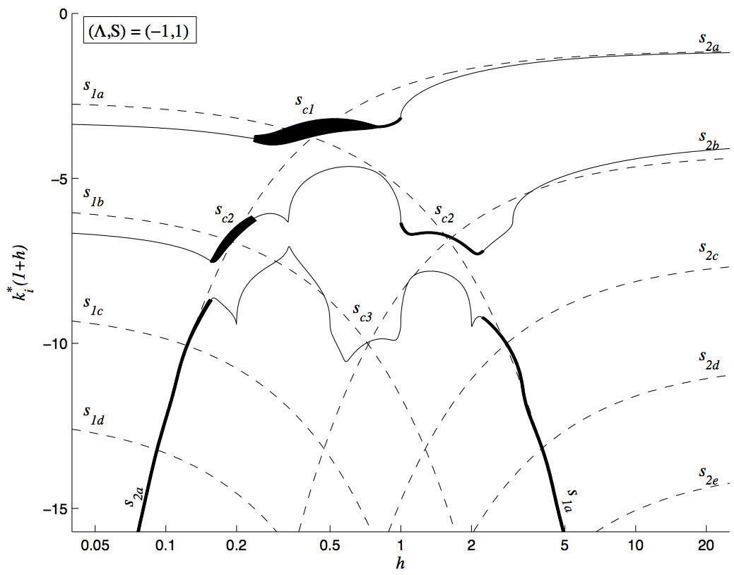
Varicose instability of confined flows
Cross-stream wavenumber (k_i) of the most unstable wave with zero group velocity as a function of confinement ratio, h, for varicose motion of a confined wake flow. The thickness of the line is proportional to the growth rate. The dashed lines show the value of k_i for modes in the inner flow and outer flow if the other flow were not present. This shows that the confined flow is most unstable at values of h at which the modes in the inner flow and outer flow have the same cross-stream wavenumber.
Credit: Matthew Juniper
Jump to publication (will be at top of next screen)
Credit: Matthew Juniper
Jump to publication (will be at top of next screen)
A video of shape optimization
Lorem ipsum donec id elit non mi porta gravida at eget metus Lorem ipsum donec id elit non mi porta gravida at eget metus Lorem ipsum donec id elit non mi porta gravida at eget metus Lorem ipsum donec id elit non mi porta gravida at eget metus
Credit: Jack Brewster
Credit: Jack Brewster
Global instability of a helium jet
This movie shows a helium jet discharging into air. The flow is globally unstable and oscillates at a well-defined frequency.
Credit: Larry Li
Credit: Larry Li
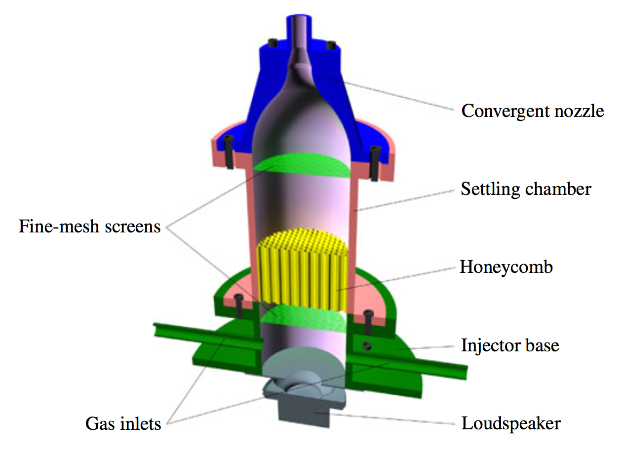
Cross-section of the low turbulence injector
This is the cross-section of the injector we used to create a jet with a nearly-flat velocity profile with turbulence intensity around 0.4%.
Credit: Larry Li
Jump to publication (will be at top of next screen)
Credit: Larry Li
Jump to publication (will be at top of next screen)
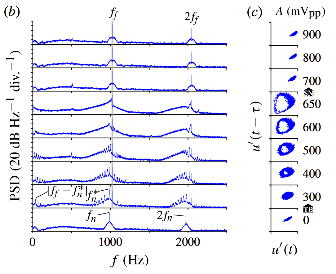
Forced response of a helium jet
Power Spectral Density (left) and Poincare map (right) of the signal from a hot wire placed inside a helium jet discharging into air. The helium jet is forced with a loudspeaker (the amplitude is shown in millivolts). At low forcing amplitudes, the transition from periodicity to quasiperiodicity occurs via a torous-birth bifurcation. At high forcing amplitudes, at which lock-in occurs, the transition from quasiperiodicity to periodicity occurs through a saddle node bifurcation with frequency-pulling.
Credit: Larry Li
Jump to publication (will be at top of next screen)
Credit: Larry Li
Jump to publication (will be at top of next screen)
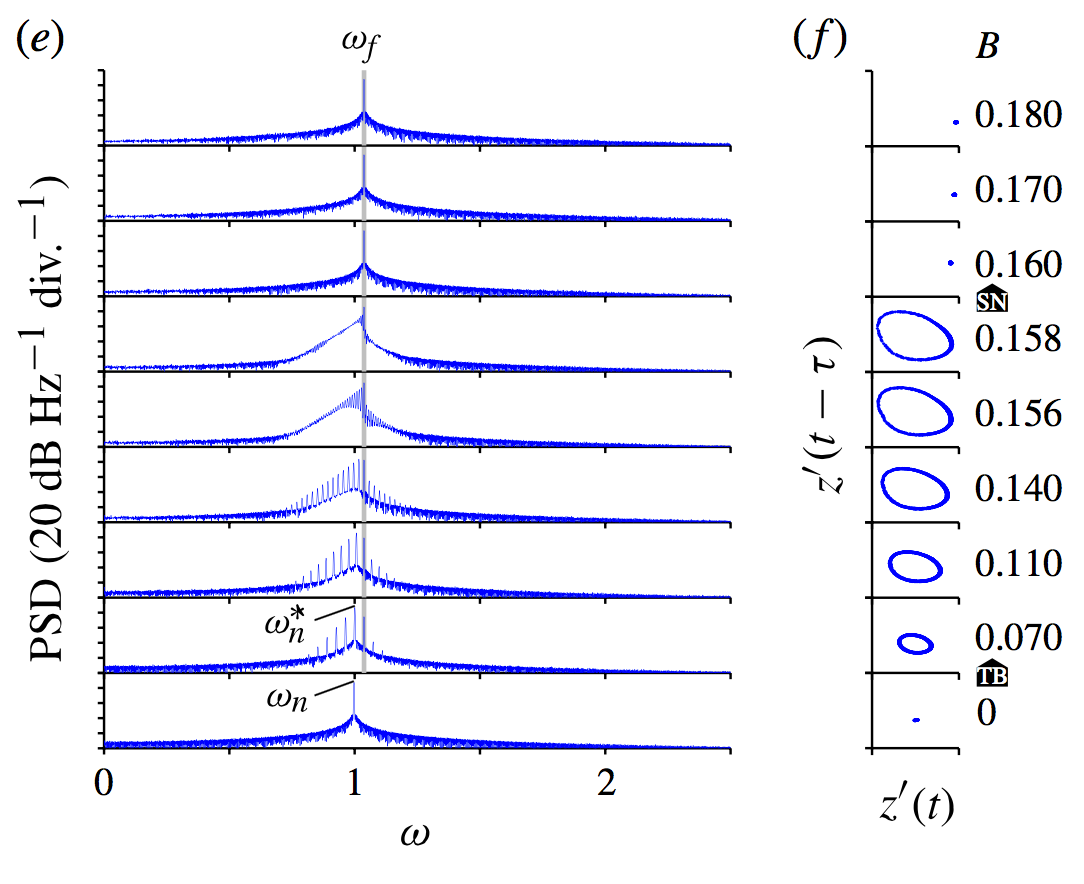
Forced response of a van der Pol oscillator
Power Spectral Density (left) and Poincare map (right) of the harmonically-forced van der Pol oscillator. At low forcing amplitudes, the transition from periodicity to quasiperiodicity occurs via a torous-birth bifurcation. At high forcing amplitudes, at which lock-in occurs, the transition from quasiperiodicity to periodicity occurs through a saddle node bifurcation with frequency-pulling. The dynamics are identical to those of the helium jet.
Credit: Larry Li
Jump to publication (will be at top of next screen)
Credit: Larry Li
Jump to publication (will be at top of next screen)
Thermoacoustic oscillations on a camping gas stove
An empty pipe is placed around the flame from a camping gas stove, causing thermo-acoustic oscillations.
Credit: Matthew Juniper
Credit: Matthew Juniper
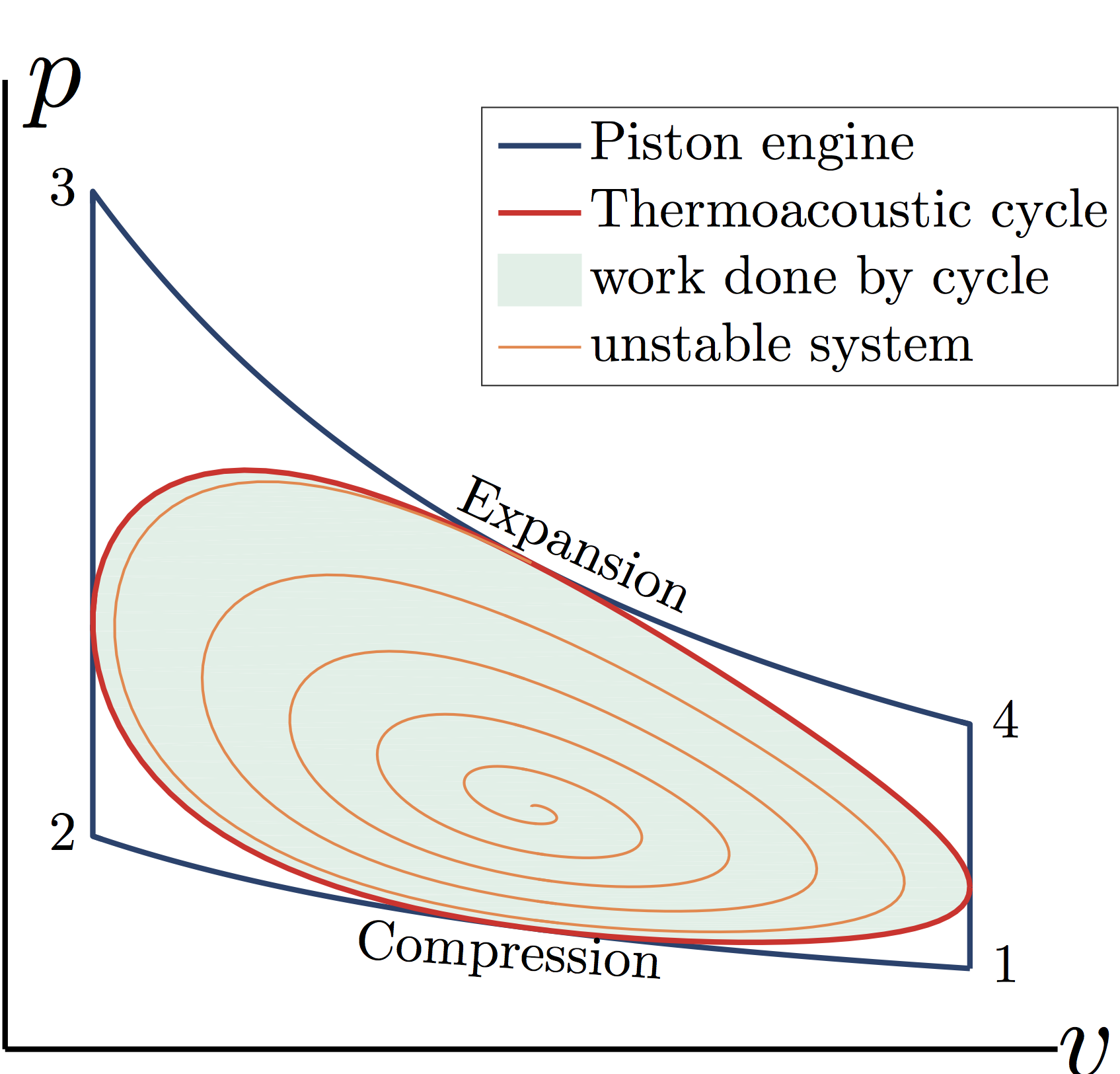
Description of the thermoacoustic mechanism via a pressure - volume diagram
The mechanism that drives thermoacoustic oscillation is similar to that which drives a piston engine. In an idealized piston engine, work is done on a gas as it is compressed isentropically from states 1 to 2 (blue compression line). From 2 to 3, the gas combusts at fixed volume, releasing heat and raising its pressure further. From 3 to 4, the gas does work as it expands isentropically (blue expansion line). More work is done by the gas during the expansion phase than is done on it during the compression phase, leading to a net conversion of heat to work given by the area within the cycle on the pressure-volume diagram. In thermoacoustics, an acoustic wave replaces the piston and a continuous flame replaces the periodically-ignited gas. The acoustic wave independently (i) perturbs this flame and (ii) compresses and expands the gas around the flame. If the perturbed flame releases more heat than average during instants of higher local pressure, then, through the same mechanism as the piston engine, more work is done by the gas during the acoustic expansion phase than is done on it during the acoustic compression phase (red cycle). If this work is not dissipated then the oscillation amplitude grows and the system is thermoacoustically unstable (orange spiral).
Credit: Matthew Juniper
Credit: Matthew Juniper
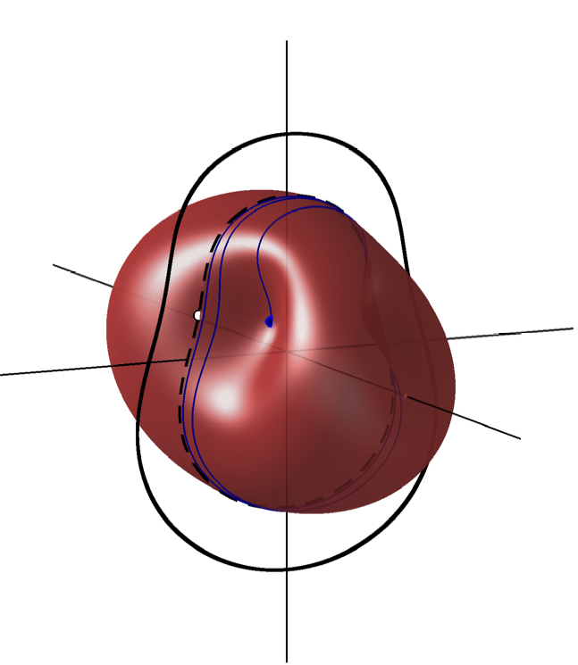
Triggering in Thermoacoustics
This is a cartoon of acoustic phase space for the thermoacoustic model used in our first investigations into triggering in the horizontal Rijke tube. The stable fixed point (the non-oscillating solution) is at the origin. The stable periodic solution (the oscillating solution) is the solid black loop. The red manifold separates the points in phase space that decay to the stable fixed point from those that are attracted to the stable periodic solution. An unstable periodic solution (dashed black line) exists exactly on the manifold. The point with lowest energy on this unstable periodic solution is marked with a white dot. Nonlinear adjoint looping is used to find points on the manifold with lower energy than this, for example the black dot. From this low energy starting point, oscillations grow to the unstable periodic solution. If they are given infinitesimally more energy initially then they grow to the stable periodic solutions. The black dot is the 'most dangerous initial state' or 'minimal seed' because it grows to stable oscillations from the lowest initial energy.
Credit: Matthew Juniper
Jump to publication (will be at top of next screen)
Credit: Matthew Juniper
Jump to publication (will be at top of next screen)
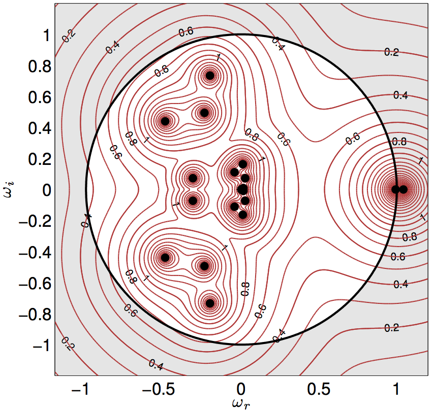
Pseudospectra of the monodromy matrix
The black dots are the eigenvalues of the monodromy matrix (also known as Floquet multipliers) describing the evolution of small perturbations around the unstable periodic solution for a thermoacoustic model of the horizontal Rijke tube. Eigenvalues that lie outside the unit circle have positive growth rate and are unstable. In this case there is a single unstable eigenvalue at omega ~ 1.05, showing that this periodic solution is unstable to perturbations with exactly the same period as the periodic solution - i.e. the amplitude of the periodic solution will grow. The red lines are the pseudospectra of the monodromy matrix. If this matrix were Hermitian (i.e. M M^T = M^T M) then its eigenvectors would be orthogonal and the pseudospectra would be the envelope of circles centred on the eigenvalues. The matrix is, however, slightly non-Hermitian, which means that the pseudospectra extend slightly further away from the eigenvalues. Physically, this means that some perturbations around the unstable limit cycle (those with omega ~ -0.2 +- 0.9i) will grow slightly before they decay. This means that the 'most dangerous initial condition' can exploit transient growth around the unstable limit cycle and therefore does not sit on the unstable periodic solution itself.
Credit: Matthew Juniper
Jump to publication (will be at top of next screen)
Credit: Matthew Juniper
Jump to publication (will be at top of next screen)
Limit cycle of a Burke-Schumann flame in a tube
This video shows a thermoacoustic limit cycle of a Burke-Schumann (diffusion) flame in a tube found using matrix-free continuation methods. The top two frames show the acoustic pressure and velocity fields in the tube. The tube has open ends so there is a pressure node and a velocity antinode at each end. The Burke-Schumann flame sits in the black box at x = 1. This field is expanded in the bottom frame. The bottom frame shows the perturbation mixture fraction field (colours) and the flame position (black line).
Credit: Iain Waugh and Simon Illingworth
Jump to publication (will be at top of next screen)
Credit: Iain Waugh and Simon Illingworth
Jump to publication (will be at top of next screen)
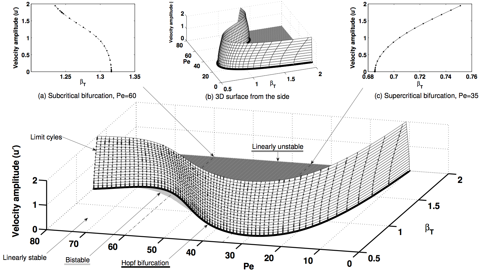
Bifurcation diagram of a Burke-Schumann flame in a tube
The bottom diagram shows the maximum velocity amplitude for limit cycles of a Burke-Schumann flame in a tube, as a function of Peclet number (Pe) and heat release parameter (beta). These are calculated with matrix-free continuation methods. The top-left frame shows a cut at Pe=60, revealing a subcritical bifurcation. The top=right frame shows a cut through Pe=30, revealing a supercritical bifurcation.
Credit: Iain Waugh and Simon Illingworth
Jump to publication (will be at top of next screen)
Credit: Iain Waugh and Simon Illingworth
Jump to publication (will be at top of next screen)
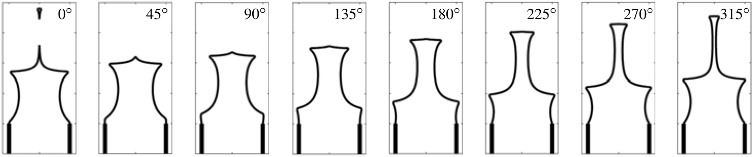
Snapshots of a harmonically-forced G-equation flame
These are snapshots of a G-equation (pre-mixed) flame when the velocity field is forced harmonically. The G-equation formulation permits the flame to wrinkle, form cusps, and pinch off.
Credit: Karthik Kashinath
Credit: Karthik Kashinath
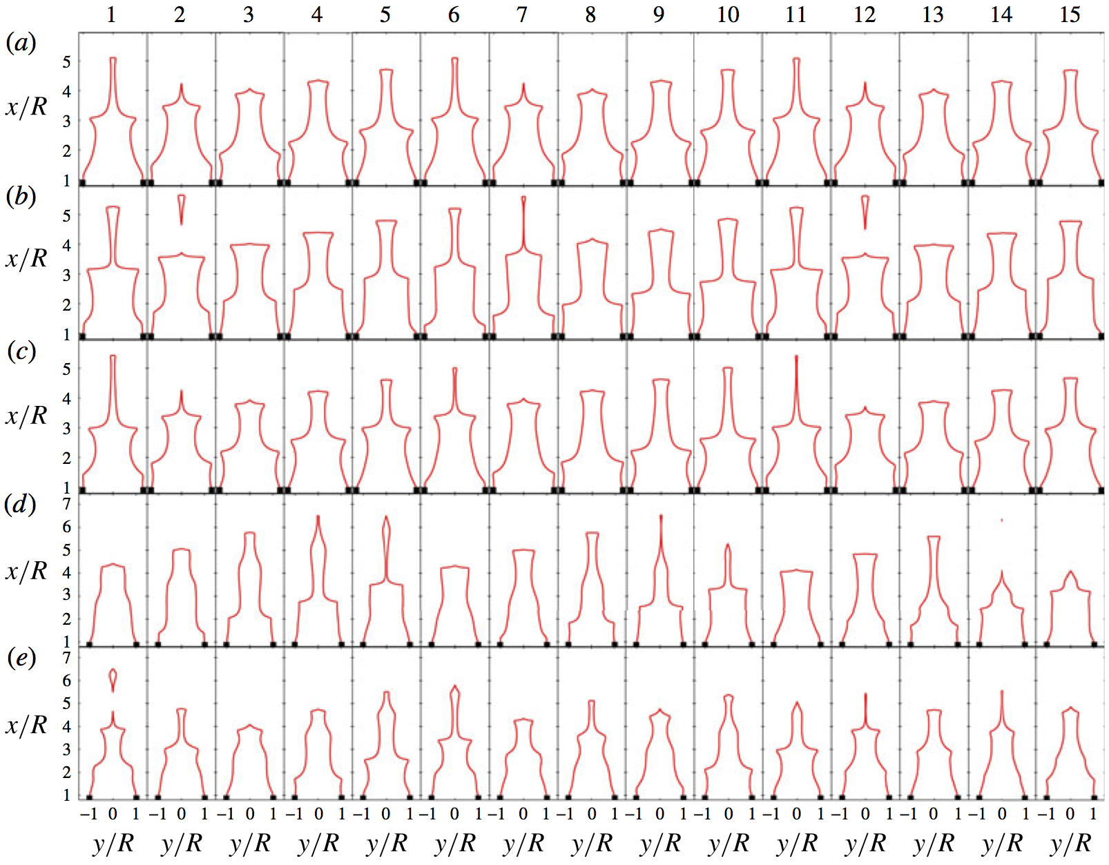
Snapshots of G-equation flames in a tube during thermo-acoustic oscillations
Each row shows snapshots of G-equation (pre-mixed) flames in a thermo-acoustically oscillating system for (a) period-1 oscillations, (b) period-2 oscillations, (c) quasi-periodic oscillations, (d) period-5 oscillations, (e) chaotic oscillations. The G-equation formulation allows simulation of flame wrinkling and pinch-off, which is required in order to simulate the elaborate nonlinear behaviour that is sometimes observed in experiments.
Credit: Karthik Kashinath
Jump to publication (will be at top of next screen)
Credit: Karthik Kashinath
Jump to publication (will be at top of next screen)
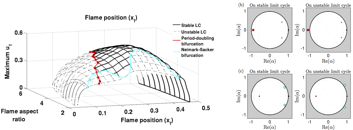
Bifurcation diagram and Floquet multipliers of a G-equation flame in a tube
The left diagram shows the bifurcation diagram for periodic thermoacoustic oscillations of a conical G-equation (premixed) bunsen flame in a tube. These oscillations are found with a continuation methods as a function of the flame aspect ratio and the flame position in the duct. The stability of these oscillations is determined by examining the Floquet multipliers, alpha. For a period-doubling bifurcation (top right), a Floquet multiplier (red dot) crosses the unit circle at alpha = -1. For a Neimark-Sacker bifurcation to quasiperiodic behaviour, a pair or Floquet multipliers (cyan dots) cross the unit circle at Im(alpha) not equal to zero. The analysis reveals that periodic solutions are often unstable.
Credit: Iain Waugh
Jump to publication (will be at top of next screen)
Credit: Iain Waugh
Jump to publication (will be at top of next screen)
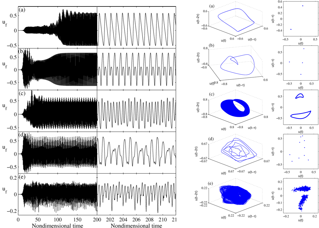
Time series data for G-equation flames in a tube during thermo-acoustic oscillations
The left figures show time series data of the acoustic velocity at the flame for a thermoacoustic oscillations of a G-equation (pre-mixed) flame in a tube. The right figures show the same information presented as phase portraits and Poincare maps. These are for (a) period 1 oscillations, (b) period 2 oscillations, (c) quasiperiodic oscillations (d) period 5 oscillations and (e) chaotic oscillations.
Credit: Karthik Kashinath
Jump to publication (will be at top of next screen)
Credit: Karthik Kashinath
Jump to publication (will be at top of next screen)
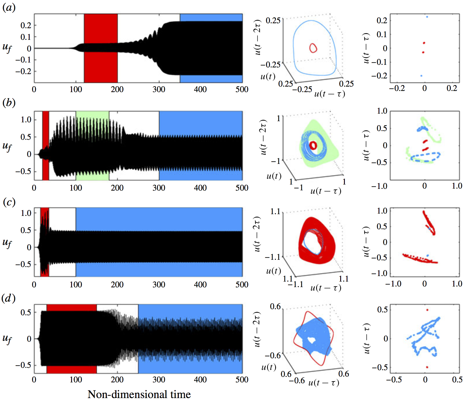
Trajectories of linearly unstable thermoacoustic systems containing G-equation flames (Fig 12)
Time series (left), phase portraits (middle), and Poincare maps (right) of the velocity signal for thermoacoustic oscillations of a G-equation flame in a tube. These show: (a) transition to a stable periodic solution (blue) via an unstable periodic solution (red), which is unstable to a quasiperiodic motion; (b) transition to a stable quasiperiodic solution (blue) via two unstable quasiperiodic solutions (blue and green); (c) transition to a stable periodic solution (blue) via an unstable quasiperiodic solution (red); (d) transition to a stable quasiperiodic solution (blue) via an unstable periodic solution (red).
Credit: Karthik Kashinath
Jump to publication (will be at top of next screen)
Credit: Karthik Kashinath
Jump to publication (will be at top of next screen)
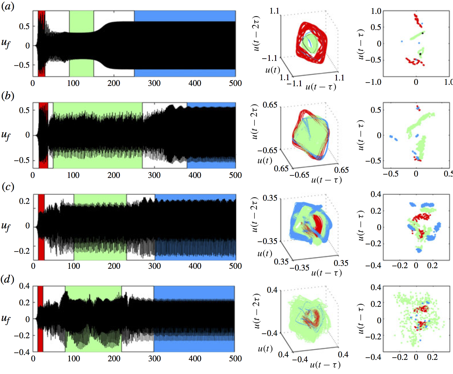
Trajectories of linearly unstable thermoacoustic systems containing G-equation flames (Fig 13)
Time series (left), phase portraits (middle), and Poincare maps (right) of the velocity signal for thermoacoustic oscillations of a G-equation flame in a tube. These show: (a) transition to a stable period 2 solution via two unstable quasiperiodic solutions (red and green); (b) transition to a stable period 2 solution via an unstable quasiperiodic solution (red) and an unstable chaotic solution (green); (c) transition to a stable chaotic solution (blue) via two unstable chaotic solutions (red and green); (d) transition to a stable period-k solution via two unstable chaotic solutions (red and green).
Credit: Karthik Kashinath
Jump to publication (will be at top of next screen)
Credit: Karthik Kashinath
Jump to publication (will be at top of next screen)
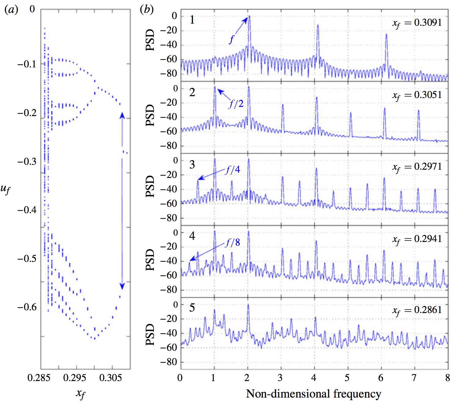
Period-doubling route to chaos observed in a thermoacoustic system containing a G-equation flame (Fig 14)
The bifurcation diagram on the left shows the negative peaks of the acoustic velocity as the location of a G-equation flame is varied within a tube. At x_f = 0.3091, these peaks pass through the same point at u_f = -0.27, showing that the solution is periodic. This can be seen clearly in the top-right figure, which shows the power spectral density (PSD) as a function of frequency. As x_f reduces, the system passes through a period-doubling bifurcation, shown by the appearance of two peaks in the bifurcation diagram and a frequency at f/2 in the PDS. A cascade of period-doubling bifurcations ensues, ending up with a chaotic oscillation.
Credit: Karthik Kashinath
Jump to publication (will be at top of next screen)
Credit: Karthik Kashinath
Jump to publication (will be at top of next screen)
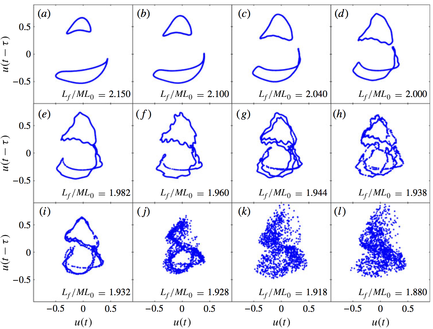
Ruelle-Takens-Newhouse route to chaos observed in a thermoacoustic system containing a G-equation flame (Fig 15)
These Poincare sections show the Ruelle-Takens-Newhouse route to chaos. The stable quasiperiodic solution in frame (a) developes corrugations on its surface due to stretching and folding. This is followed by torous breakdown to chaos.
Credit: Karthik Kashinath
Jump to publication (will be at top of next screen)
Credit: Karthik Kashinath
Jump to publication (will be at top of next screen)

Bifurcation diagram of a thermoacoustic system containing a G-equation flame (Fig 3)
This bifurcation diagram shows the peaks and troughs of acoustic velocity during thermoacoustic oscillations of a G-equation flame in a duct. The bifurcation parameter, x_f, is the position of the flame within the duct, from 0 at the entrance to 0.5 at the mid-point.
Credit: Karthik Kashinath
Jump to publication (will be at top of next screen)
Credit: Karthik Kashinath
Jump to publication (will be at top of next screen)
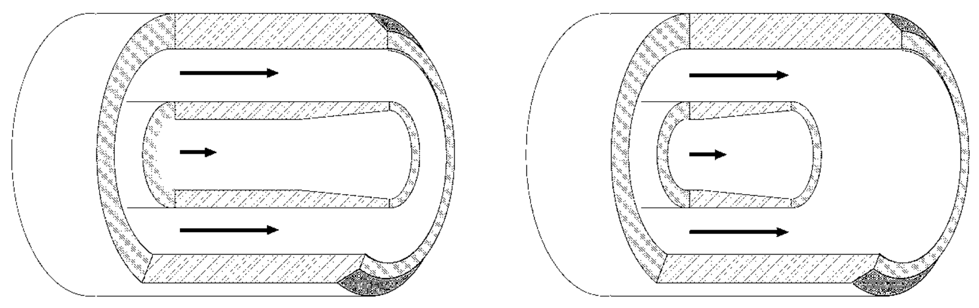
Recessed coaxial injector
Rocket engines often use coaxial fuel injectors, in which liquid Oxygen is injected through the central tube while gaseous hydrogen is injected through the outer annulus. Experiments show that the combustion efficiency improves if the central tube is recessed within the outer tube.
Credit: Matthew Juniper
Jump to publication (will be at top of next screen)
Credit: Matthew Juniper
Jump to publication (will be at top of next screen)
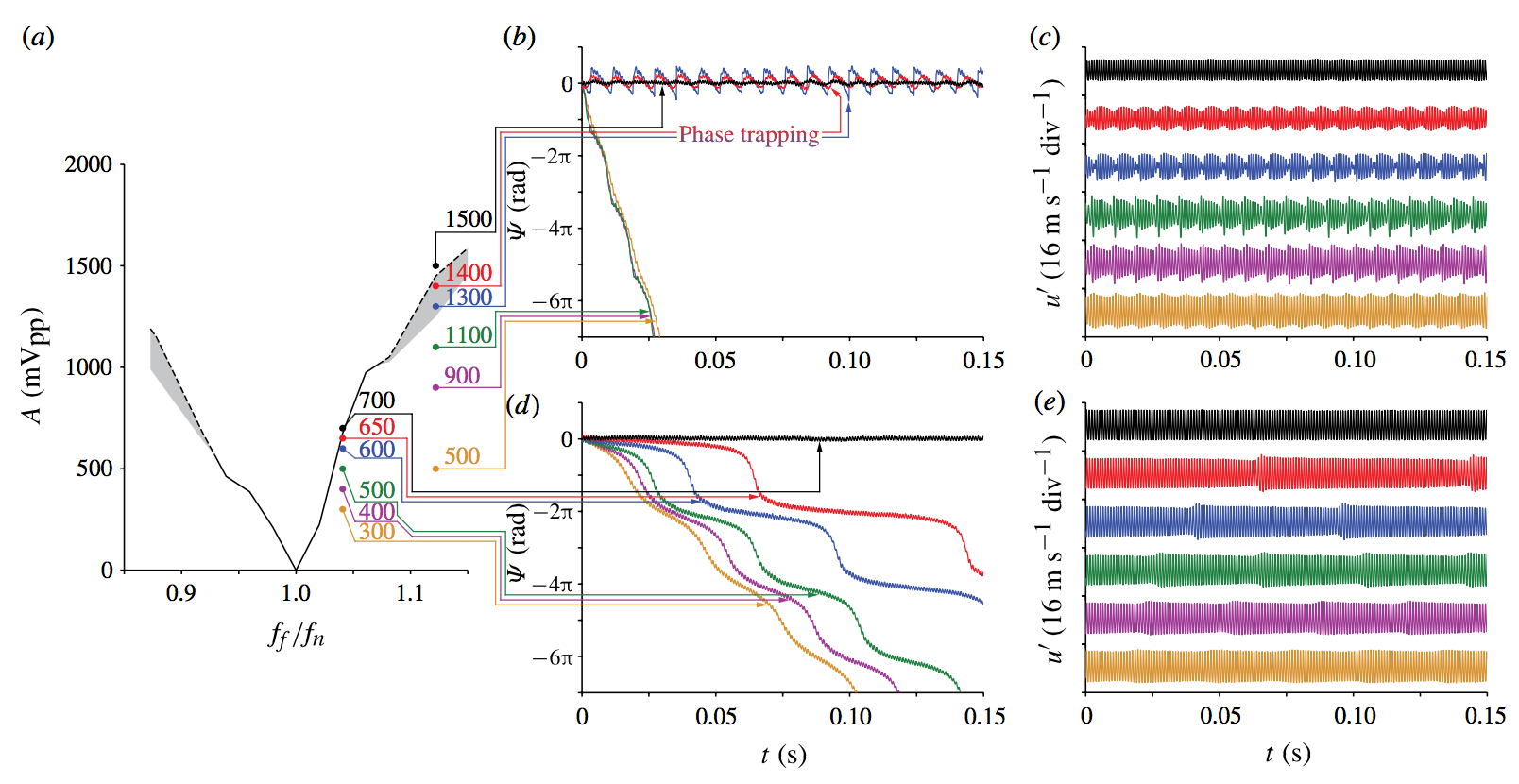
Phase trapping and slipping in a forced helium jet
Experimental data from a forced helium jet. Top-right: time series data at high forcing amplitudes, where phase trapping occurs above a forcing amplitude of 1300 mV. Bottom-right: time series data at low forcing amplitudes, where phase slipping occurs below a forcing amplitude of 700 mV. The phase trapping and phase slipping regimes (centre) can be plotted on the synchronization diagram (left) and are compared with that of a forced van der Pol oscillator in our paper on the subject.
Credit: Larry Li
Jump to publication (will be at top of next screen)
Credit: Larry Li
Jump to publication (will be at top of next screen)
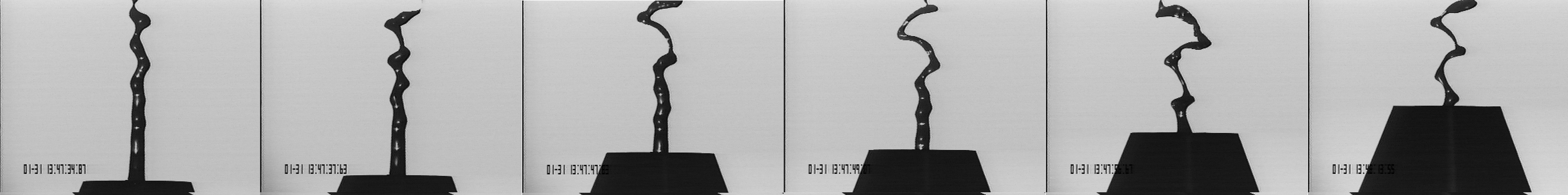
Effect of confinement
These images show a coaxial injector consisting of a slow-moving water stream within a fast-moving air stream. The tube ejecting water remains stationary as the tube ejecting air is extended downstream of it. This creates a region of confined flow just downstream of the water injector, which enhances the wake-like oscillation that can be seen in the water jet
Credit: Matthew Juniper
Credit: Matthew Juniper
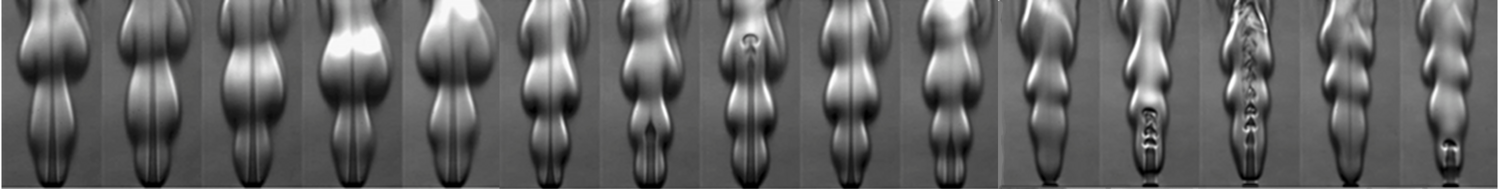
Schlieren image of a forced methane jet diffusion flame
This jet diffusion flame oscillates naturally at 12 Hz. Here, it is forced at 17 Hz with forcing amplitudes of 20% of the mean jet velocity (first five images), then 50% (second five images) and 100% (last five images). At high forcing amplitudes, the flame's oscillations lock into the forcing frequency. We found, however, that the natural mode re-appears downstream.
Credit: Larry Li
Jump to publication (will be at top of next screen)
Credit: Larry Li
Jump to publication (will be at top of next screen)