What is Flow-MRI?
Flow-MRI is an experimental technique that visualizes 3-dimensional 3-component velocity fields in opaque flows such as blood. The images are noisy, so acquisition times tend to be long in order to average out the noise. Adjoint-accelerated Bayesian inference applied to Flow-MRI data could reduce Flow-MRI scan times by a factor of 100 compared with standard methods and a factor of 10 compared with state-of-the-art compressed sensing. This will potentially transform access to clinical Flow-MRI, which is used to assess cardiovascular disease, the greatest cause of death worldwide.
How we sharpen Flow-MRI images
Our method of physics-enhanced velocimetry (PEV) increases the spatial resolution and removes the noise by using prior knowledge that the image is of fluid flowing through a tube and must therefore satisfy a Navier-Stokes boundary value problem. We use adjoint-accelerated Bayesian inference to infer the parameters of a Navier-Stokes boundary value problem expressed as partial differential equations solved with a Finite Element Method.
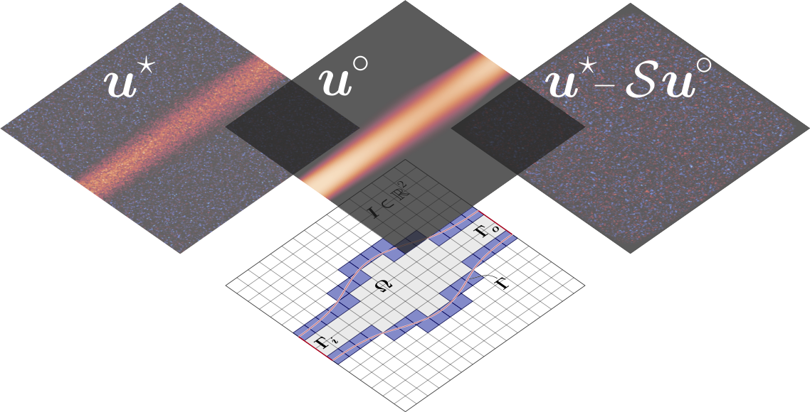
We infer the flow by creating a Navier-Stokes boundary value problem whose tunable parameters define the boundary's shape, Γ, the inlet velocity profiles, u(Γi), and the viscosity. Using adjoint methods, we calculate the derivatives of the velocity field, u, with respect to all the parameters. We then use gradient-based optimization to find the parameters that minimize the discrepancy between the modelled, u◦, and experimental, u*, velocity fields.
2D steady experimental data
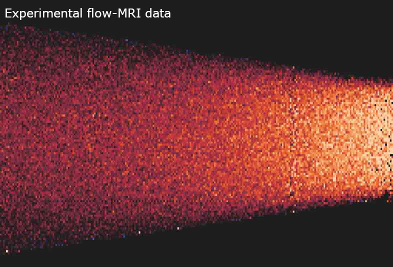
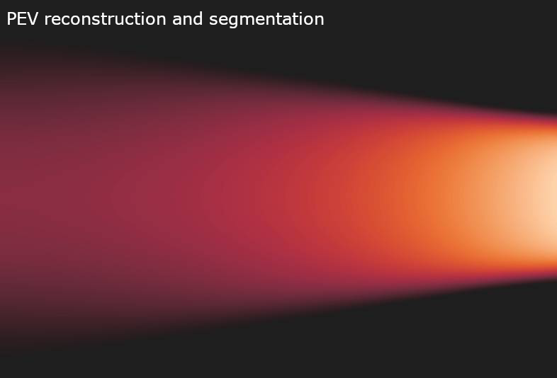
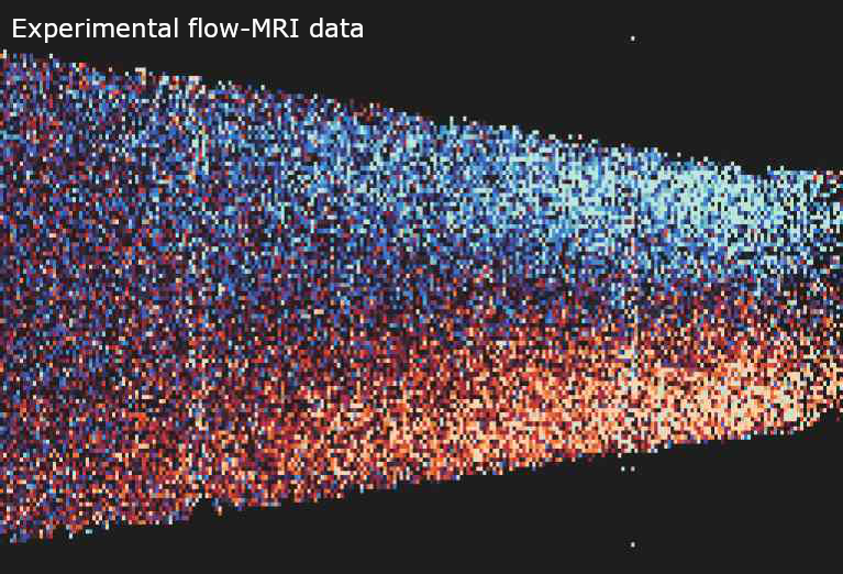
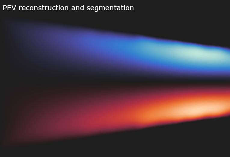
Hover over or tap the images below to see PEV applied to experimental flow-MRI data of flow through a nozzle:
Horizontal velocity magnitude of flow through a nozzle (hover over or tap to see PEV reconstruction and segmentation)
Vertical velocity magnitude of flow through a nozzle (hover over or tap to see PEV reconstruction and segmentation)
2D steady synthetic data
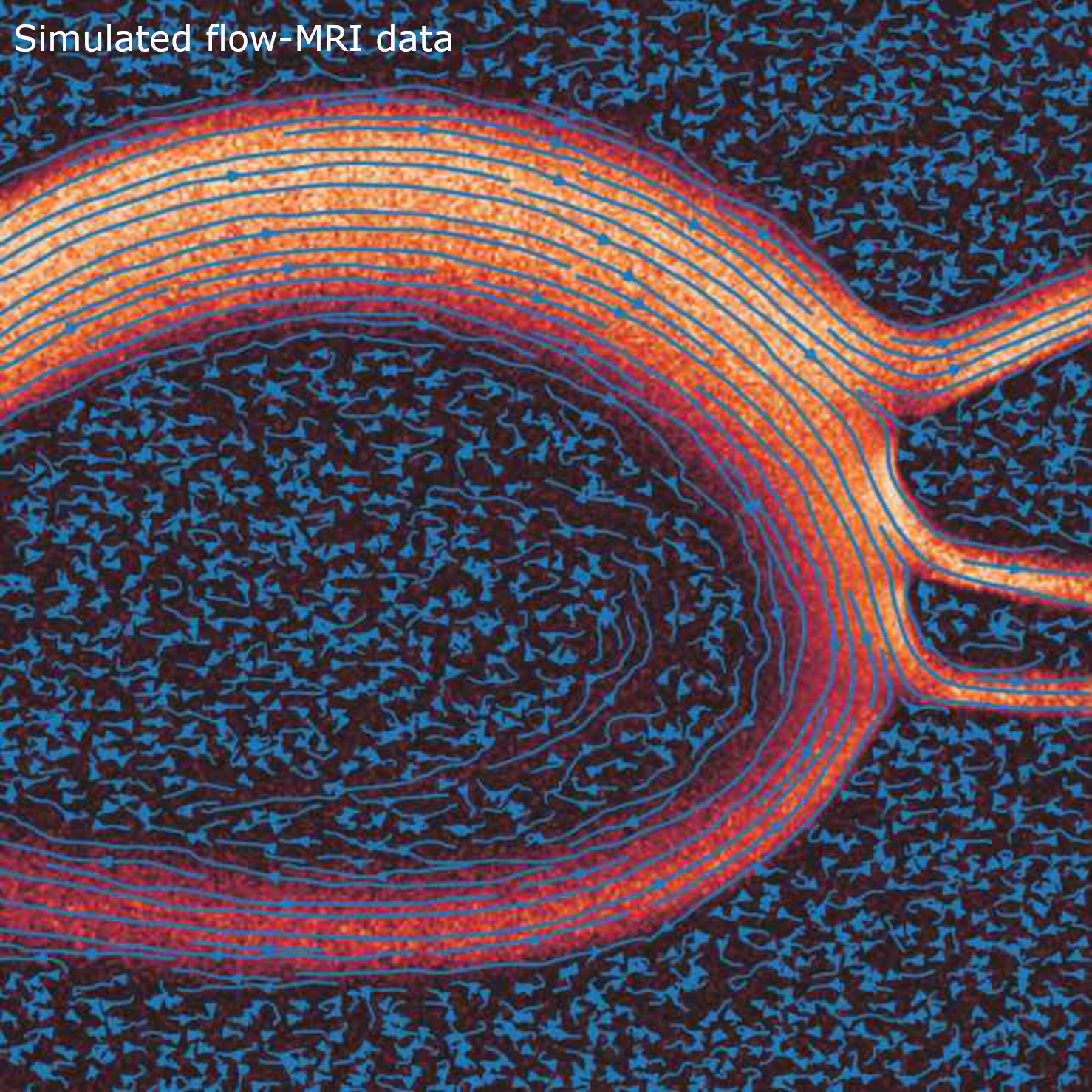
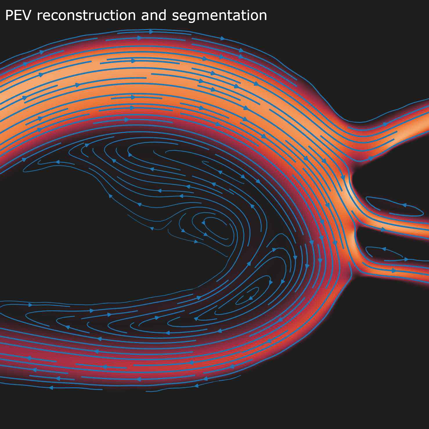
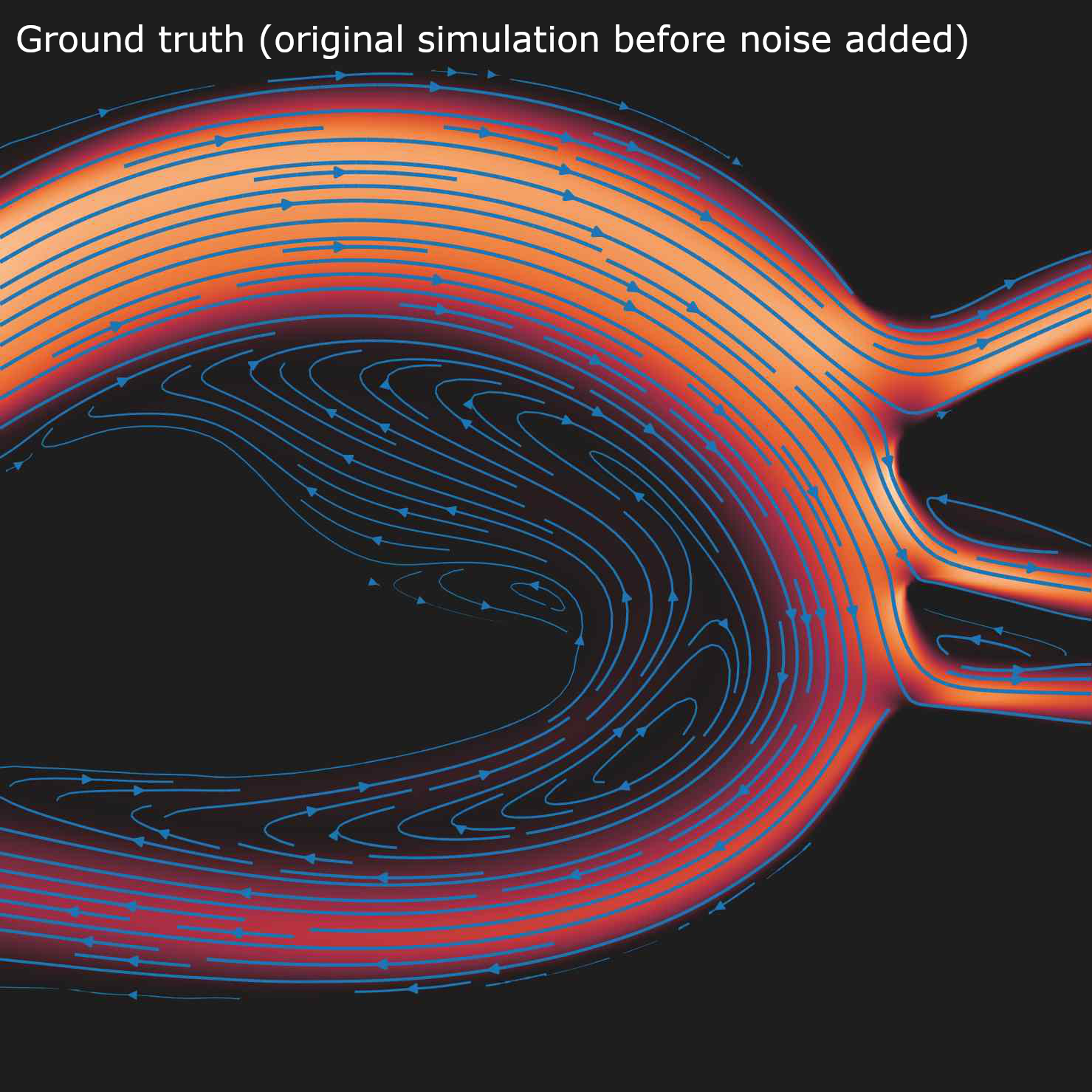
The boundary position is inferred from the velocity field, and vice-versa, meaning that the boundary and the flow are always consistent with each other. We use an immersed boundary method, which means that arbitrarily complex boundaries can be considered. Hover over the images below to see PEV applied to synthetic flow-MRI data of flow through an aorta. The comparison with ground truth shows how well our method can extract the original flow from the noisy data:
Streamlines and velocity magnitude of simulated flow-MRI image of through an aorta (hover over or tap to see PEV reconstruction and segmentation
Streamlines and velocity magnitude of the original simulation (ground truth for the PEV reconstruction and segmentation)
A common misconception is that we achieve this with a physics-informed Neural Network (PINN), which is not the case. The PINN approach assimilates data into a neural network with many more degrees of freedom than our model, applying the Navier–Stokes equations as a soft constraint. In other words, PINNs search a larger parameter space and then penalise flows & boundaries that do not satisfy the Navier–Stokes equations, while we search a small parameter space that is already hard-wired to satisfy the Navier–Stokes equations. Both methods require calculation of the gradients of each model with respect to its parameters. PINNs calculate these through automatic differentiation. We calculate these through adjoint methods and shape sensitivity. We have experimented with PINNs but our physics-based adjoint method is better.
Compared with PINNs, our approach is faster and more accurate, is physically-interpretable, can predict flows it has not seen or modelled before, and does not suffer from AI hallucinations and the fact that there is not always a stable training algorithm. Full details can be found in our first paper on the subject:
Joint reconstruction and segmentation of noisy velocity images as an inverse Navier–Stokes problem
A. Kontogiannis, S. V. Elgersma, A. J. Sederman, and M. P. Juniper
Journal of Fluid Mechanics 944 (A40) (2022) doi:10.1017/jfm.2022.503
pdf
Open Access
doi: https://doi.org/10.1017/jfm.2022.503
arXiv
We formulate and solve a generalized inverse Navier–Stokes problem for the joint velocity field reconstruction and boundary segmentation of noisy flow velocity images. To regularize the problem we use a Bayesian framework with Gaussian random fields. This allows us to estimate the uncertainties of the unknowns by approximating their posterior covariance with a quasi-Newton method. We first test the method for synthetic noisy images of 2D flows and observe that the method successfully reconstructs and segments the noisy synthetic images with a signal-to-noise ratio (SNR) of 3. Then we conduct a magnetic resonance velocimetry (MRV) experiment to acquire images of an axisymmetric flow for low (~6) and high (> 30) SNRs. We show that the method is capable of reconstructing and segmenting the low SNR images, producing noiseless velocity fields and a smooth segmentation, with negligible errors compared with the high SNR images. This amounts to a reduction of the total scanning time by a factor of 27. At the same time, the method provides additional knowledge about the physics of the flow (e.g. pressure), and addresses the shortcomings of MRV (low spatial resolution and partial volume effect) that otherwise hinder the accurate estimation of wall shear stresses. Although the implementation of the method is restricted to 2D steady planar and axisymmetric flows, the formulation applies immediately to 3D steady flows and naturally extends to 3D periodic and unsteady flows.
3D steady experimental data
We have repeated this process for experimental flow-MRI images through a 3D-printed aorta. The raw data can be downloaded with the paper below.
Bayesian inverse Navier-Stokes problems: joint flow field reconstruction and parameter learning
A. Kontogiannis, S. V. Elgersma, A. J. Sederman, M. P. Juniper
Inverse Problems 41 015008 (2025) doi:10.1088/1361-6420/ad9cb7
pdf
Open Access
doi: https://doi.org/10.1088/1361-6420/ad9cb7
3D Flow-MRI low SNR data (Python npy binary files)
arXiv
We formulate and solve a Bayesian inverse Navier-Stokes (N-S) problem that assimilates velocimetry data in order to jointly reconstruct a 3D flow field and learn the unknown N-S parameters, including the boundary position. By hardwiring a generalised N-S problem, and regularising its unknown parameters using Gaussian prior distributions, we learn the most likely parameters in a collapsed search space. The most likely flow field reconstruction is then the N-S solution that corresponds to the learned parameters. We develop the method in the variational setting and use a stabilised Nitsche weak form of the N-S problem that permits the control of all N-S parameters. To regularise the inferred the geometry, we use a viscous signed distance field (vSDF) as an auxiliary variable, which is given as the solution of a viscous Eikonal boundary value problem. We devise an algorithm that solves this inverse problem, and numerically implement it using an adjoint-consistent stabilised cut-cell finite element method. We then use this method to reconstruct magnetic resonance velocimetry (flow-MRI) data of a 3D steady laminar flow through a physical model of an aortic arch for two different Reynolds numbers and signal-to-noise ratio (SNR) levels (low/high). We find that the method can accurately i) reconstruct the low SNR data by filtering out the noise/artefacts and recovering flow features that are obscured by noise, and ii) reproduce the high SNR data without overfitting. Although the framework that we develop applies to 3D steady laminar flows in complex geometries, it readily extends to time-dependent laminar and Reynolds-averaged turbulent flows, as well as non-Newtonian (e.g. viscoelastic) fluids.
Physics-informed compressed sensing
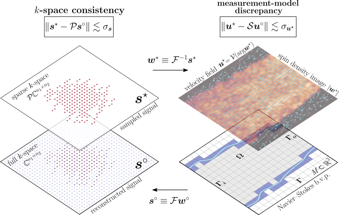
In flow-MRI, the raw signal from the sensors is received in wavenumber space (k-space). This space is often sub-sampled in order to reduce the amount of data required for a given amount of information. We combine PEV and Compressed Sensing in a method known as Physics-Informed Compressed Sensing (PICS). This uses prior knowledge that the image is of flow through a tube to decompress the signal and remove noise simultaneously.

Graphical representation of physics-informed compressed sensing (PICS)
Given the sparse k-space data, s*, corresponding to a measured velocity field, we solve an inverse Navier–Stokes problem to infer the boundary Γ, the kinematic viscosity, and the inlet velocity profile on Γi. The solution to this inverse problem is a reconstructed signal, s◦, corresponding to a calculated velocity field, which is simultaneously de-noised, un-wrapped, and segmented.
Credit: Alexandros Kontogiannis
Jump to publication (will be at top of next screen)
This simultaneously de-noises, unwraps, and segments the image, extracting the same amount of information from hundreds of times less data than standard flow-MRI.
Physics-informed compressed sensing for PC-MRI: an inverse Navier-Stokes problem
A. Kontogiannis and M. P. Juniper
IEEE Transactions on Image Processing 32 281--294 (2022) doi:10.1109/TIP.2022.3228172
pdf
Open Access
doi: https://doi.org/10.1109/TIP.2022.3228172
arXiv
We formulate a physics-informed compressed sensing (PICS) method for the reconstruction of velocity fields from noisy and sparse phase-contrast magnetic resonance signals. The method solves an inverse Navier–Stokes boundary value problem, which permits us to jointly reconstruct and segment the velocity field, and at the same time infer hidden quantities such as the hydrodynamic pressure and the wall shear stress. Using a Bayesian framework, we regularize the problem by introducing a priori information about the unknown parameters in the form of Gaussian random fields. This prior information is updated using the Navier–Stokes problem, an energy-based segmentation functional, and by requiring that the reconstruction is consistent with the k-space signals. We create an algorithm that solves this reconstruction problem, and test it for noisy and sparse k-space signals of the flow through a converging nozzle. We find that the method is capable of reconstructing and segmenting the velocity fields from sparsely-sampled (15% k-space coverage), low (~10) signal-to-noise ratio (SNR) signals, and that the reconstructed velocity field compares well with that derived from fully-sampled (100% k-space coverage) high (>40) SNR signals of the same flow.

